Udacity Self-Driving Car Nanodegree Project 8 - Kidnapped Vehicle

The eighth project for the Udacity Self-Driving Car Engineer Nanodegree Program, and the third for Term 2, was titled “Kidnapped Vehicle” but that name was more or less window dressing on top of what was in many ways another take on the concepts of the previous two projects (The Extended Kalman Filter project and the Unscented Kalman Filter project). All three are primarily concerned with taking noisy, uncertain sensor measurements and movements, and combining them to produce a more precise state belief (whether that state is the location, orientation, and velocity of a pedestrian, a bicyclist, or, in this case, our own vehicle).

While the Kalman Filter projects involved fusing measurements from radar and LiDAR sensors to locate a single obstacle from our vehicle’s perspective, the goal of the Kidnapped Vehicle project was to find our own vehicle’s uncertain location in a known, mapped area with known ground truth landmark locations, LiDAR data representing the observed location of landmarks in relation to the vehicle, and vehicle control data. So, last time we had multiple sensors and a single observation for each frame (the pedestrian or bicyclist) and this time we have a single sensor and multiple observations for each frame. The tool we were tasked to accomplish this with was the inimitable particle filter.

This wasn’t my first time to tango with a particle filter. Six months ago, I wrote about my experience taking Udacity’s Artificial Intelligence for Robotics course, which included a unit on particle filters. Here’s what I had to say about them back then:

The particle filter also operates in continuous environments, but it’s a bit more of a shotgun, guess-and-check localization method. You basically take a massive number of random guesses at where you are and where you’re heading (copies of your robot), then take a measurement and “resample”, which means that bad guesses drop out and good guesses are duplicated (and better guesses are duplicated even more). This move-measure-resample sequence is repeated until the guesses converge and you’re left with a bunch of copies of the absolute best guess.

Now that I’ve stewed over the Kalman and particle filters a bit longer, I’ve come to realize that they do essentially the same thing - they just approach it differently. The Kalman filter bakes the uncertainty into our best-guess state by representing it as a multidimensional Gaussian - it’s a single belief stretched out to encompass a wide area (in 2D, for example), whereas the particle filter actually peppers a number of discrete copies of that best guess over pretty much that same area. Weird, huh? Both methods then predict the future state belief of the Gaussian/particles and update that belief based on measurement data.

For some time I wondered how the particle filter can possibly improve once we’ve pared down to a single particle. If the original distribution of particles is sparse enough, we’d quickly converge to a single particle. And if the best particle in the original set turned out to have a significant error, won’t that error just persist as we copy that particle over and over? Well, I wasn’t taking into account the motion noise. You see, even if we kill off all but one particle, in the very next step the hundred or thousand (or however many) copies of that particle are going to fan out in different directions. The spread of that fan is going to depend on the built-in motion noise, and I’d be willing to bet that with enough particles the resulting distribution just might resemble that Gaussian we would have had using a Kalman filter (assuming our motion noise is Gaussian). Cool!

This project was a bit more open-ended than the previous two Kalman filter projects. We were given method stubs for init, prediction, dataAssociation, updateWeights, and resample and we had far less code from lesson material available to copy over, so there was a lot of room to maneuver, so to speak. The prediction method accepts motion data and predicts the new location for each particle based on the data, and resample simply drops and duplicates particles based on their weights. updateWeights required the most thought - it accepts a list of landmarks and observations, and our job is to associate observations with landmarks based on the particle pose and calculate the weight for each particle (which is determined by how closely those observations, transformed into map coordinates, correspond to landmark locations within sensor range). My first stab at it looked something like this:

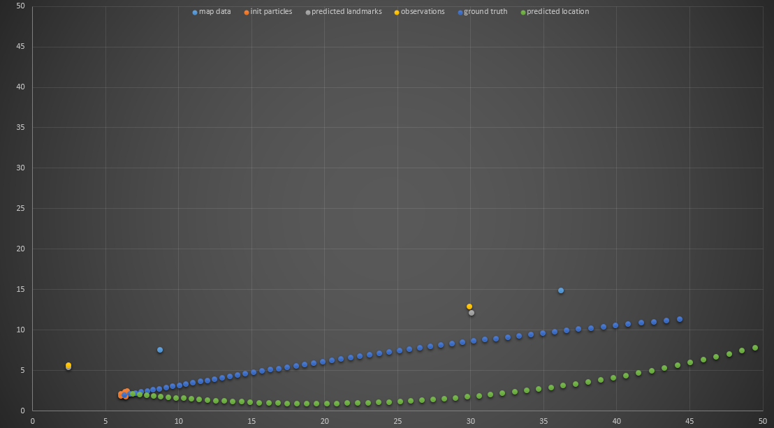
I knew I was on the right track since the transformed observations (yellow dots) were near the landmarks (blue dots), but there was obviously something wrong because my best particle quickly got off track. I tested my resample method and was confident it worked, so I suspected it was an issue with my prediction method. I found one minor bug, but it still wasn’t working correctly:

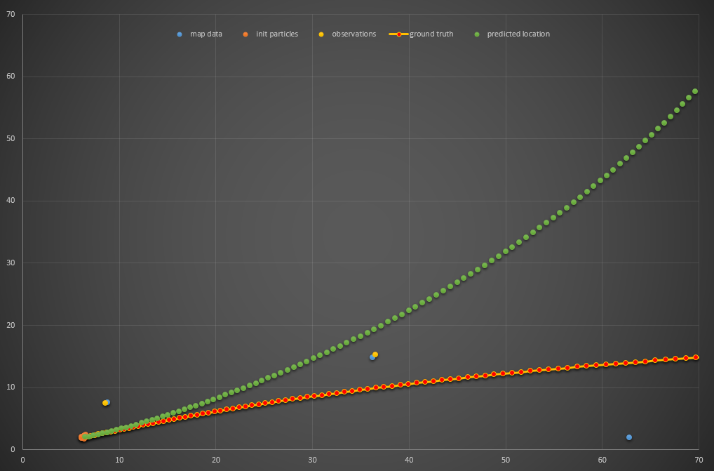
Notice that the observations and “predicted landmarks” (gray dots) are reasonably close, but the particle motion is still wrong. I decided the culprit had to be my updateWeights method. The way I implemented it at first was to transform the nearby landmarks (blue dots) into the particles’ coordinates, so I recoded updateWeights almost entirely so that the observations are instead transformed to the map’s coordinates before the associations and weights are determined. This did the trick and the particle filter was working like a charm.

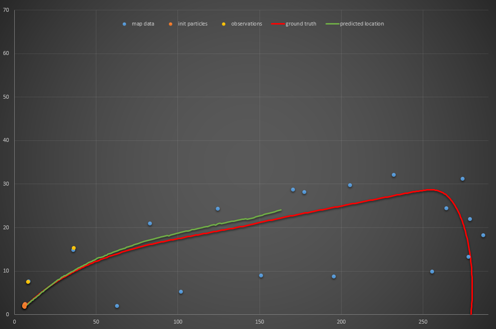
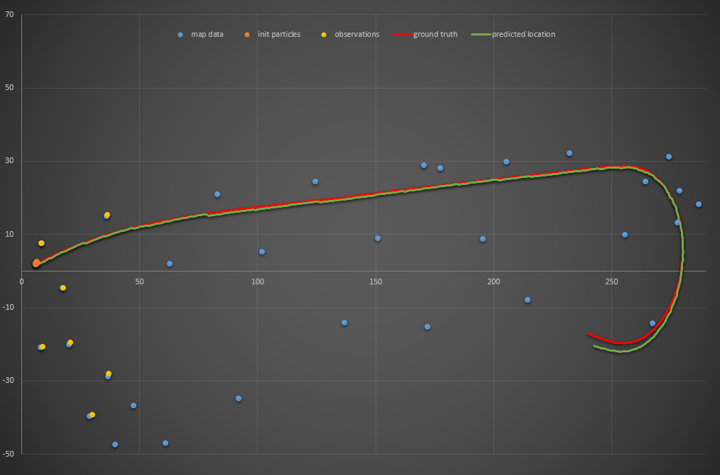
Since the project rubric dictated that compute time was of the essence, I wanted to see how few particles I could use and still get a reliable filter. Here’s a single particle which quickly diverges, as you might expect:

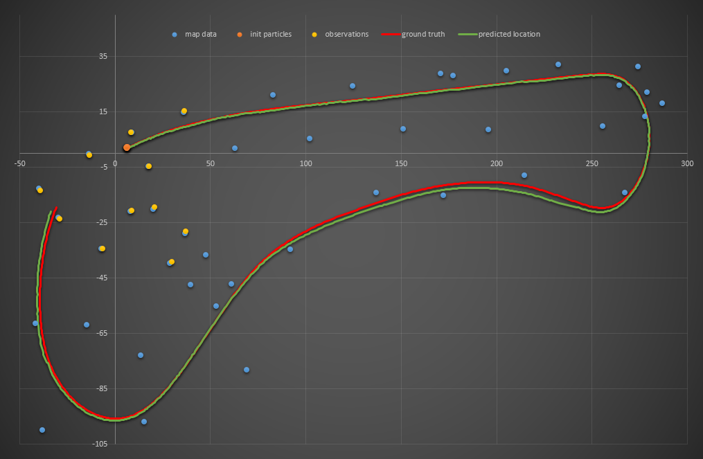
Two particles fared far better (I realize the chart cuts off, but I assure you it didn’t continue much further):

Three particles:

Four particles:

Five particles:

Six particles:

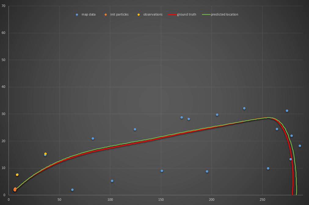
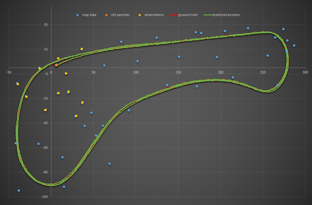
Success! It actually traces that NSFW shape a few times. I ran the code no less than twenty times and it was successful every single time. I pumped my fist and submitted my project for review. Turns out, that was a dumb idea. It was returned “does not meet specifications” because, for the reviewer, it failed… and for the same reason that my two-particle filter performed better than my three-particle filter: the noise you use to initiate your particles means (especially when you’re only using a few particles) you might just get lucky with one that performs especially well. My six-particle solution worked time after time because I was using the same random seed to generate those six particles every time and one just happened to work. The reviewer generated a different initial six particles, and they all failed.

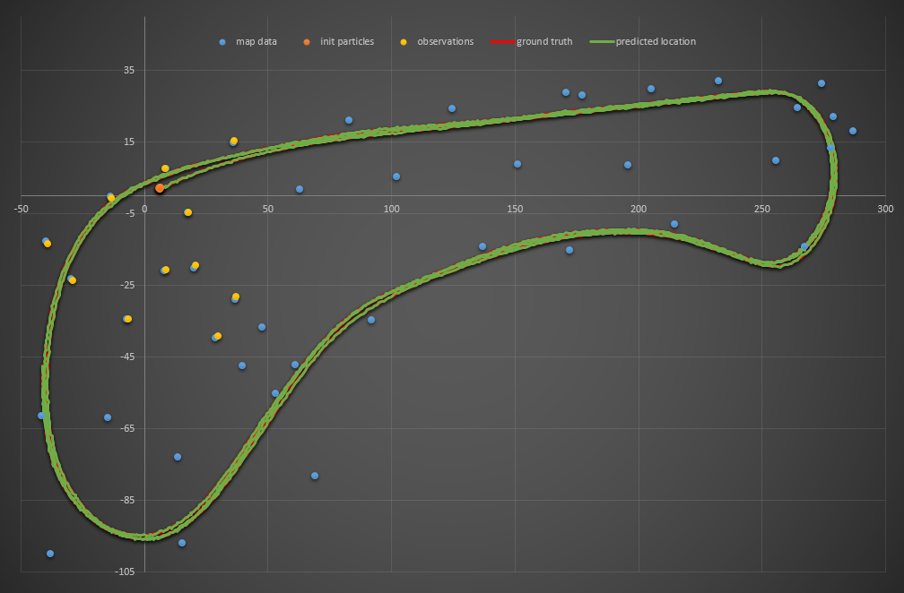
Of course, I didn’t really mean (believe it or not) to submit my project with just six particles. I resubmitted with 101…

…and passed!

The source code for this project can be found on my GitHub