Udacity Self-Driving Car Nanodegree Project 6 - Extended Kalman Filter

Term 2 of the Udacity Self-Driving Car Engineer Nanodegree Program is in full swing. The pace thus far is more relaxed than Term 1 (which is welcome since I’m also on a team competing in the Didi Challenge), but the difficulty has been dialed up a couple of notches. Maybe it’s the C++, maybe it’s the math, maybe it’s the Didi Challenge, or maybe all of the best students were quietly snatched up Rapture-style by hiring partners, but the Slack channels and the Facebook groups are noticeably quieter since Term 1 ended. I can only assume that most students, after being exposed to the Kalman Filter - the subject of the first Term 2 project, are scratching their heads and wondering “WTF is going on with this?!” Because that’s how I reacted on my first encounter with it.

Well, I’ll try to shed some light on my understanding of Kalman Filters. I can’t claim to have the firmest grasp on it, so… grain of salt, here. But maybe you’ll find my perspective helpful to refine your own.

In a perfect world, everything works exactly as expected. And when you build a robot and tell it to go forward one meter, it does exactly that. And then when you pull out your Righteous Measuring Tape of Exactitude you find that, indeed by the grace of the lord almighty, it moved forward exactly one meter. Praise be! He is risen!

Well I’ve got news for you, sister - it don’t work like that. I don’t care how careful you were when you built it, that robot didn’t move exactly one meter. And while I’m bursting bubbles, I may as well let you know that your measurement was off. Maybe not by much (if you bought the expensive measuring tape), but I guarantee it was off.

Well, crap! That just made my easy problem (determining that robot’s location) a lot harder. But hold on a sec! Enter: Gaussians. Magical, magical Gaussians.

Beautiful, is it not? Here’s the equation for that little bump:

The Gaussian is completely defined by its mean (or “expected value” - the actual measured value, represented by the symbol mu in the equation, which looks like the letter u) and variance (the uncertainty of the measurement, represented by sigma, which looks like an o) - the larger the variance, the wider the bump. The true magical beauty of Gaussians happens when you combine them. The product of two Gaussians? A Gaussian. The convolution of two Gaussians? Again, a Gaussian. The Fourier Transform of a Gaussian? You guessed it - a Gaussian. See for yourself.

That means that we don’t have to worry so much about the e’s and square roots and pi’s, and can focus just on the u’s and o’s, making the calculations far simpler. When you get into trying to work with complex movements and measurements in multidimensional space, this trick is a lifesaver. I can’t imagine that the actual probability distributions for any robot’s motion or any sensor’s measurement follow a Gaussian distribution, necessarily, but they’re just so dang easy to work with that it’s worth it to assume they do.

So that’s basically what we’re doing with the Kalman Filter - taking just the mean and variance for each dimension of our robot’s motion that we’re interested in tracking and putting them into a “state” vector and “covariance” matrix, respectively. From there, the math is relatively simple. It’s just a cycle of predict (“based on your previous motion, I’d expect you to be here n seconds later”) and measurement update (“but my sensor thinks you’re here”), from which a compromise is made and a new state vector and covariance matrix are determined. This is all contained in a short list of equations, which I am not going to get into right now (this post is already long enough). The Extended Kalman Filter simply adapts these equations slightly to account for nonlinear relationships between current/previous states and states/measurements.

Phew! How about an example?

These are the two sets of sensor measurements (in yellow), and associated ground truth (in blue) given for the project, along with my Kalman Filter estimate (in green):

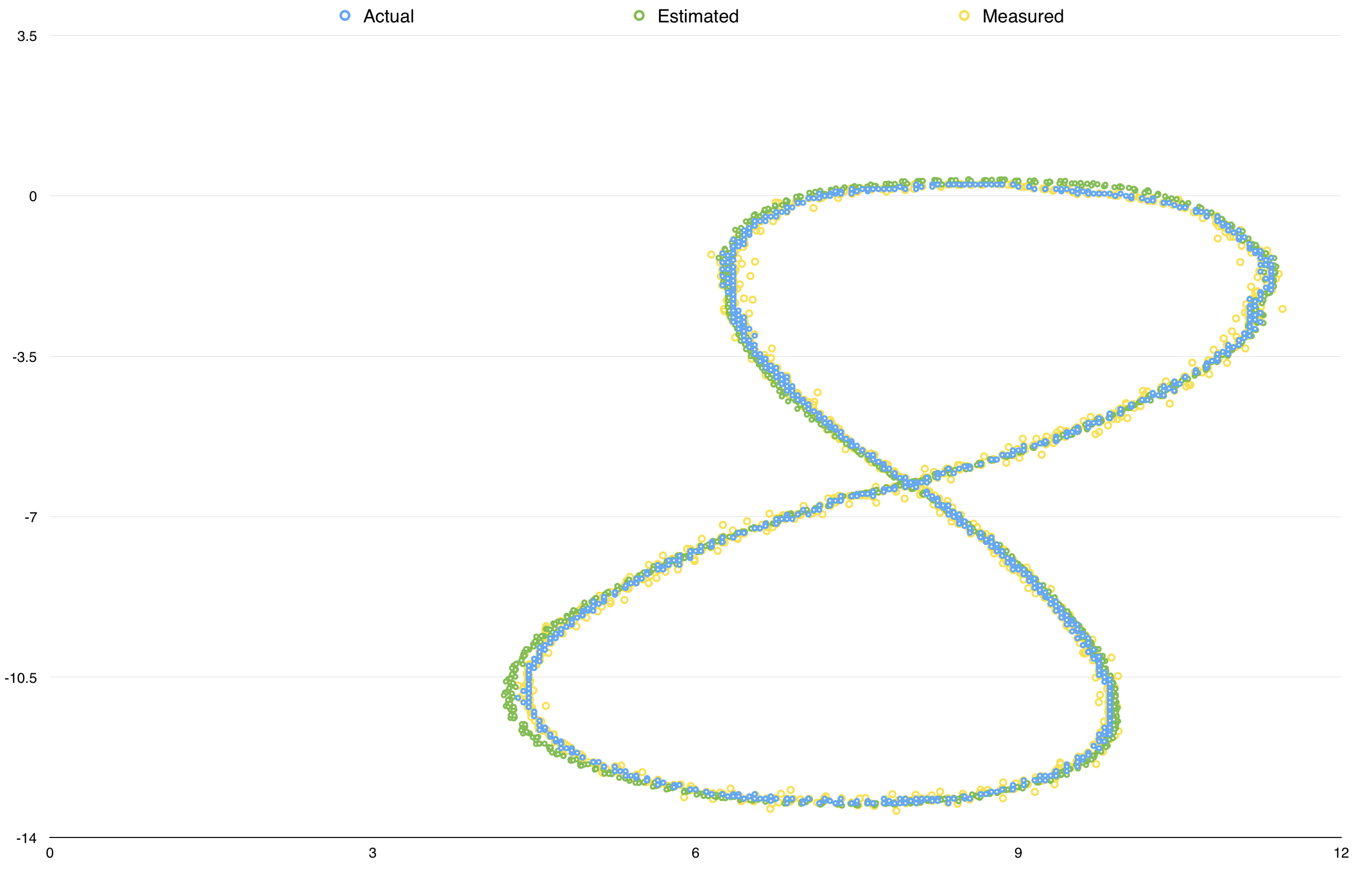
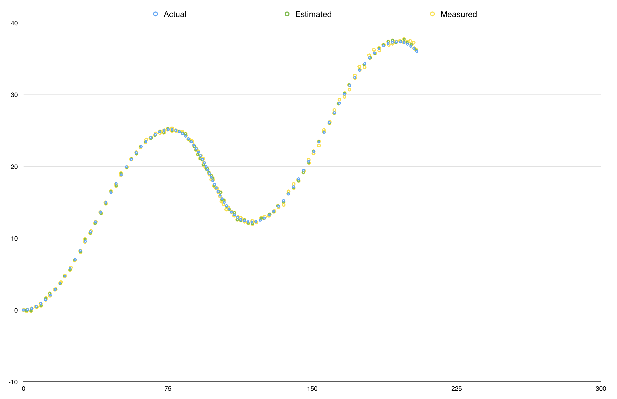
The measurements came from both LiDAR and radar measurements. The challenge was adapting the Kalman Filter to interpret both types of measurements, because while the LiDAR measurements conform to the (Euclidean) parameters of our state vector, the radar measurements use polar coordinates and require a conversion between coordinate systems (and, hence, the Extended Kalman Filter).

The source code for this project is available on my Github here.