DiDi Just Hear You Say 'Challenge'? (Part 1)

This is part one of a (probably) two-part series reflecting on my experience in the Udacity DiDi Challenge

When the DiDi Challenge was announced, I wasn’t sure if I should invest my time in it. Months earlier, between the announcement of the Nanodegree and the beginning of Term 1, Udacity held a series of competitions for which thousands signed up but I imagine (if the DiDi Challenge is any indication) only a few dozen followed through. I abstained because I was so focused on completing as many of the Nanodegree’s suggested prerequisite courses as possible before beginning Term 1, and didn’t want to bog myself down trying to jump too far ahead. This time, though, I was feeling more confident, I had some time to spare before Term 2 began, and a team was conveniently soliciting teammates in the Facebook group. I cautiously offered to dedicate a minimal five hours per week - my priority was still first with the Nanodegree and second with this blog that you’re reading.

The team quickly grew to over forty members, but just as quickly solidified into a core of four or five of us who regularly joined the Skype meetings. We were at a significant disadvantage because none of us had experience with ROS, PCL, or the KITTI Benchmark Suite (the inspiration for the DiDi Challenge). We spent an inordinate amount of time just trying to understand what the heck the goal of the challenge was and how to get there with the data provided. To further complicate things, turnover at Udacity meant that there were some hiccups in the rollout of the challenge - datasets had to be rereleased, deadlines pushed back, requirements clarified. Some teams became frustrated and I suspect more than one quit in protest, but I wasn’t phased - I wasn’t in it to win the $100k prize money; I just wanted to learn some ROS and PCL. (Spoiler alert: I did!)

Several of us downloaded the ROSbag datasets and explored them using rviz. But this is as far as some of us got, due mainly to Nanodegree/university obligations and/or technical difficulties. In the meantime, I began Term 2 and ordered a hardcopy of the fantastic A Gentle Introduction to ROS. It was Nanodegree lectures and projects during the day, and then a few pages of this book in bed before falling asleep. I’d have to work on the challenge between Nanodegree projects.

Udacity provided several snippets of code to help with things like parsing the ROSbags, generating tracklet files (the deliverable, basically XML), and a ROS node to process point cloud data. I struggled mightily to run this ROS node - for whatever reason (probably several reasons, really) I could not seem to get the node to compile using catkin_make. But then, Eureka! I’m not sure what combination of circumstances led to it, but I was now running it. I had one terminal running roscore, another running rosbag play -l whatever_the_bag_name_was.bag, another running the Velodyne driver node to convert the bag’s velodyne_packets to velodyne_points using the command rosrun velodyne_pointcloud cloud_node _calibration:=/opt/ros/indigo/share/velodyne_pointcloud/params/32db.yaml, and finally Udacity’s ROS-examples node rosrun lidar lidar_node which produced something like this:

(disregard that mouse pointer) The team rejoiced. Progress!

The original node produced an overhead view of the LiDAR points (as you can see), saved it to disk, and published this view as a point cloud on a different ROS topic. I shelved the saving and publishing, and decided to start simple: let’s draw a little circle around the LiDAR position. There was a nice helper method to convert point cloud X,Y coordinates to image coordinates, so I gave it a (0,0) and called cv::circle. Easy enough.

From here, I explored the /objects/obs1/rear/gps/rtkfix ROS topic. This is what differentiated the DiDi Challenge from KITTI. You see, the KITTI dataset is hand-labeled with the ground truth bounding boxes contained in tracklet files. Udacity/DiDi took a different approach - because hand labeling is slow and expensive, they stuck a precison GPS receiver on the (single) obstacle car and gave us its RTK coordinates, and those of the capture car, to establish the ground truth. The first dataset was flawed because it was impossible to establish the position of the obstacle car relative to the capture car (because both RTK coordinates were in relation to a GPS base station). They solved this by adding a second GPS transmitter to the capture car, which could be used to establish its orientation. This is what the setup looked like:

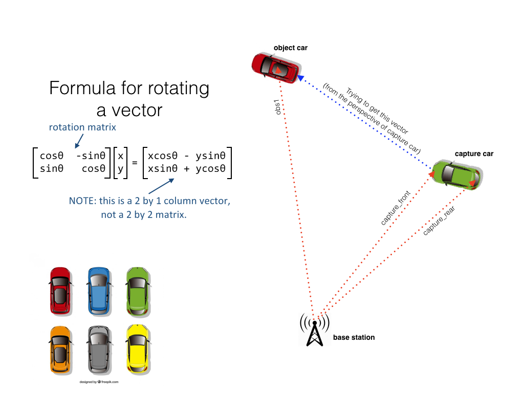
I took the three RTK coordinates (relative to the base station) and the equations listed, and in just a few lines of code added another circle - this time onto the obstacle car.

(disregard that errant circle - I fixed that later) Not bad! I was genuniely surprised to see this work on the first attempt. Does that ever happen to you? You think something is going to be a pain to code and then it magically works. I dunno - it makes me feel like I cheated or something… anywho!

Now it was time to get fancy with PCL. I started with this tutorial on cluster extraction and made changes to suit this particular application. It conveniently combines several pieces that lead up to the extraction of clusters of points from the point cloud, including downsampling the cloud using a voxel grid and ground plane segmentation and removal. I added conditional removal of points above and below certain Z heights (where we wouldn’t expect to see the obstacle car anyway) and, later, of points corresponding to the capture car. Tuning the clustering parameters was the most difficult part, but here is the final result before removing the capture car:

And after:

• White circles = centroids of clusters
• Pink circle = obstacle car RTK location
• Cyan circle = LiDAR location

The final step was to compute the centroids of the clusters. I could use these centroids to determine whether the cluster belongs to the obstacle car or not based on its proximity to the obstacle car RTK coordinates. Using this approach, I built a dataset of “car” and “noncar” images by extracting 64x64 squares of pixels around the centroids. I had considered building a classifier for the raw point cloud clusters, partly because I discovered the PCL library includes an SVMClassifier class! Here’s why I decided against it, though, as described to my teammates:

I’ve been stewing on this for a couple of days, and I don’t think I can build a classifier on raw point cloud cluster data. The main reason, I’m thinking, is because most (all?) ML algorithms require your input data shape to be consistent. With these point clouds, though, when the clusters are distant they might have only 10 points, and when they’re close they might have 100 or more. There might be ways to work around that, and maybe the PCL SVMClassifier is one way to do it - I just don’t think I have time to figure it out and I can’t seem to find a single example of it out on the Internet.

So I guess my plan from this point is: convert N x N patches of the point cloud, centered at the cluster centroid, to a height map image (just like is being displayed in the video, but maybe a 64x64 square), save these little images to ‘car’ and ‘notCar’ folders, and then we can build a classifier on those suckers (one of you people with a nice GPU). :) Thoughts?

Here’s a smattering of some of the image files that this produced:

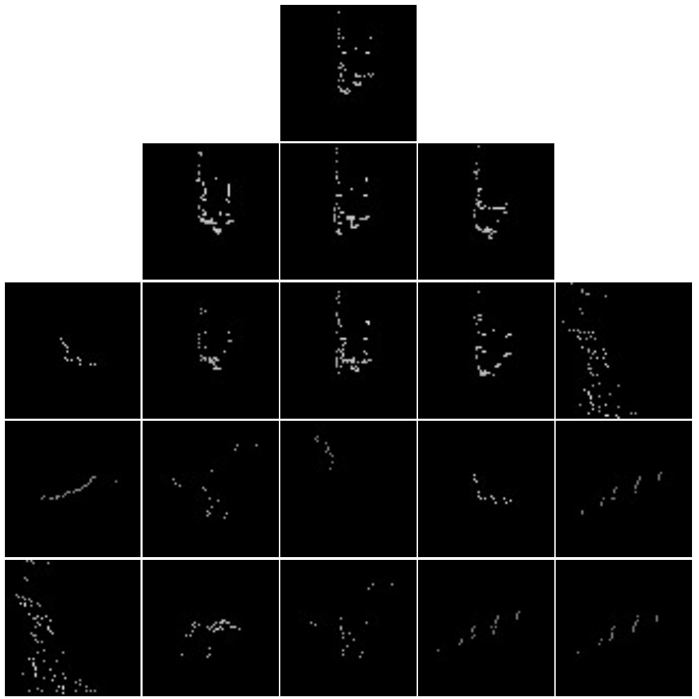
Can you guess which are cars and which aren’t? How about which ones are little dinosaurs?

This brings us to only a few days before the competition deadline, and it’s what I threw together in those last few days that I plan to share in Part 2. Stay tuned!

Feel free to skip ahead and check out the code on GitHub if you want (you’ll be missing out on all my charm, though).

Update! Part two is now available!