Udacity Self-Driving Car Nanodegree Project 7 - Unscented Kalman Filter

Today is my wife’s birthday (What’s up, Sexay? Happy birthday!), so I’m dedicating this blog post to her. I guess maybe it’s fitting, uh… given her mild obsession with unconventional deodorants? OK, that’s a stretch (especially considering they’re rarely unscented) but, whatever - this one’s for you, babe!

In our last turgid episode, I was extolling the virtues of the Gaussian distribution. This post isn’t exactly a departure from that main point, and I doubt you’re surprised to find that the Unscented Kalman Filter project didn’t turn out too very unlike the Extended Kalman Filter project. The differences were essentially twofold: of course there were the inherent differences between the EKF and UKF themselves, but also instead of tracking a hypothetical pedestrian, this time we were tracking a hypothetical cyclist. For that reason we introduced a new motion model: Constant Turn Rate and Velocity, or CTRV.

The motion model we used for the pedestrian in the EKF project was the Constant Velocity (CV) model, which was only concerned with the position (in x and y dimensions) and velocity (also in x and y dimensions) of the pedestrian being tracked. This model assumes that if the pedestrian is in motion, it will continue to move in that way from one moment to the next, and any change in that motion (i.e. acceleration) is modeled by the “process noise.” Bicycles don’t move like pedestrians do, though. The CTRV model trades the x and y components of the velocity for a direction and magnitude, and adds in a “yaw rate” component - the change in heading from one moment to the next. If you think about it, this makes sense - when riding a bike you might not change the angle of your handle bars very much from moment to moment, and even though your velocity might be constant your heading will be changing (i.e. you’ll have a constant yaw rate). This motion model will help to reduce error in our tracking algorithm.

There are other motion models out there, such as Constant Turn Rate and Acceleration (CTRA) and Constant Curvature and Acceleration (CCA) which introduce additional state parameters and frankly complicate the hell out of your state transition matrix. This paper goes over some of the advantages and disadvantages of the CV, CTRV, CTRA, and CCA models for tracking a vehicle’s location. They find, unsurprisingly, that the models perform similarly for highway driving, but that in an urban setting the more complex motion models outperform the simpler ones. Obviously, the motion model you should choose just depends on your situation.

In the EKF blog post, I mentioned briefly that the EKF accounts for nonlinear relationships between our state vector and the measurement vector, or for the state vector between time steps. For example, if my state space includes x and y position and my sensor measures exactly that or some linear variation of it then we’re all good - I can use the plain ol’ Kalman Filter because the measurement-to-state transition is linear and (remember?) when you put a Gaussian into a linear system you get a Gaussian out. But what if my radar measures distance and angle, which means the measurement-to-state transition matrix includes sin and cos? In that case the EKF uses a Taylor expansion to come up with a linear approximation of the transition function. It ain’t perfect, but it gets the job done.

The UKF takes a different approach - and it doesn’t require any of that disgusting calculus BS, so rejoice! What it does is kind of so stupidly simple I’m still in disbelief that it actually works. The plain Kalman Filter passes the state mean through a transition function (different for predict or update steps) and out spits the new state mean. Well, the UKF just picks out a few other points (strategically, depending on the dimensionality of the state space), called “sigma points”, and passes them through the same transition function. Now, since our transition function is nonlinear, those points might not spit out as evenly spaced as they were before, but that’s OK. We just let them pull the mean their direction a bit, and in the end we’ve got our new mean state space. We can even add our process noise into the mix - just dump it all in there and turn the crank. The covariance works in about the same way and is derived pretty simply based on the difference between the new state mean and the predicted (post-transition) sigma points. Essentially, we’re fitting a new Gaussian to the output of our transition function, and we’re still reducing what would probably be an incredibly complex, five-dimensional probability distribution into a single state vector and single covariance matrix. Gaussians save the day once again!

Another minor aspect that made the UKF project different from the EKF project was that we weren’t given values for our process noise. This noise was divided into two orthogonal vectors: the acceleration in the direction of the velocity vector, and the acceleration in the yaw direction. I won’t spoil it for others who want to tune their noise parameters, but the object is to get the “normalized innovation squared” (NIS) - a measure of how noisy your actual measurements are in terms of how noisy you expect them to be based on your covariance - to conform to a “Chi-squared distribution”. WTF, right? How about a picture?

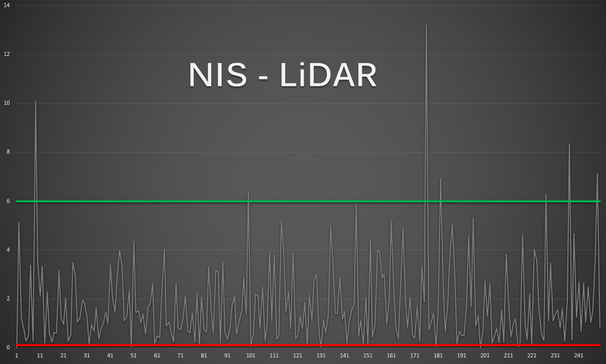
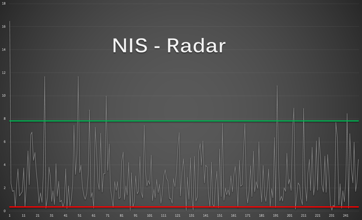
All we’re looking for is that around 90% of the points stay between those red and green lines. That’s just for the LiDAR measurements, and the one below is for the radar measurements.

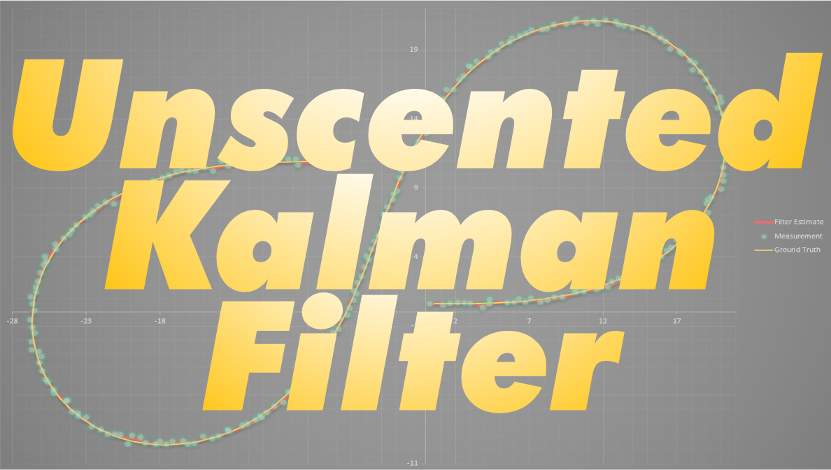
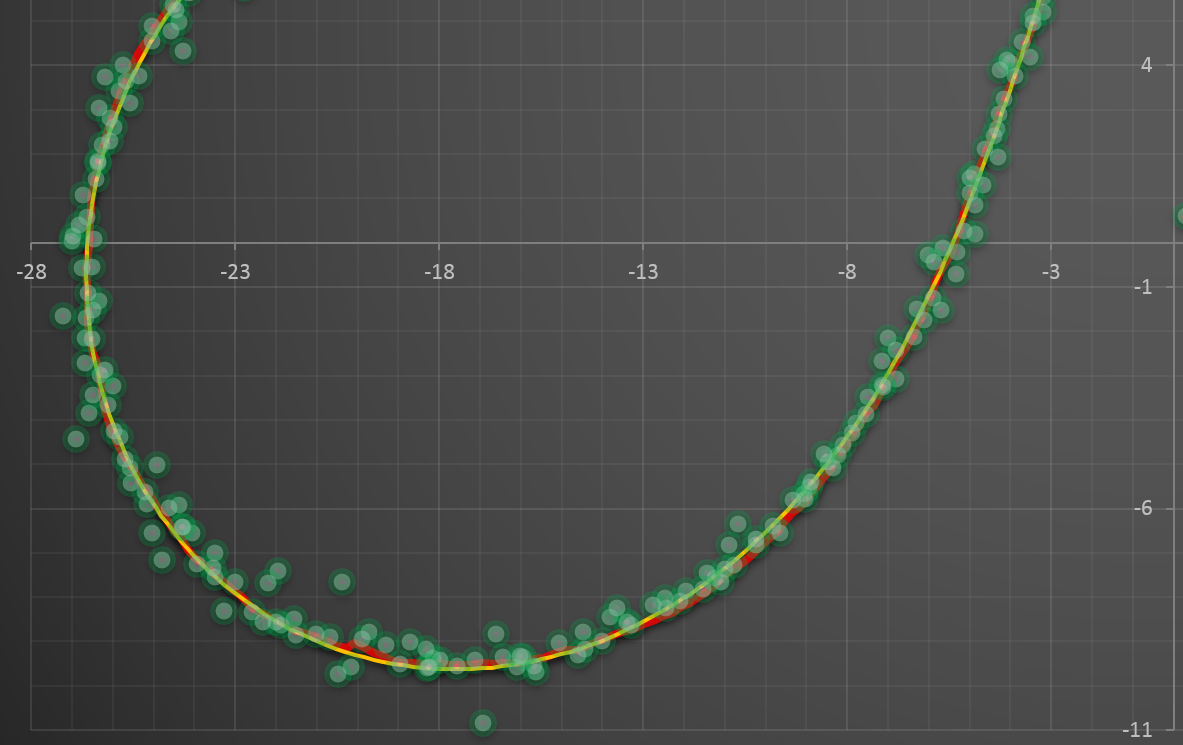
Here’s the final output of my Unscented Kalman Filter:

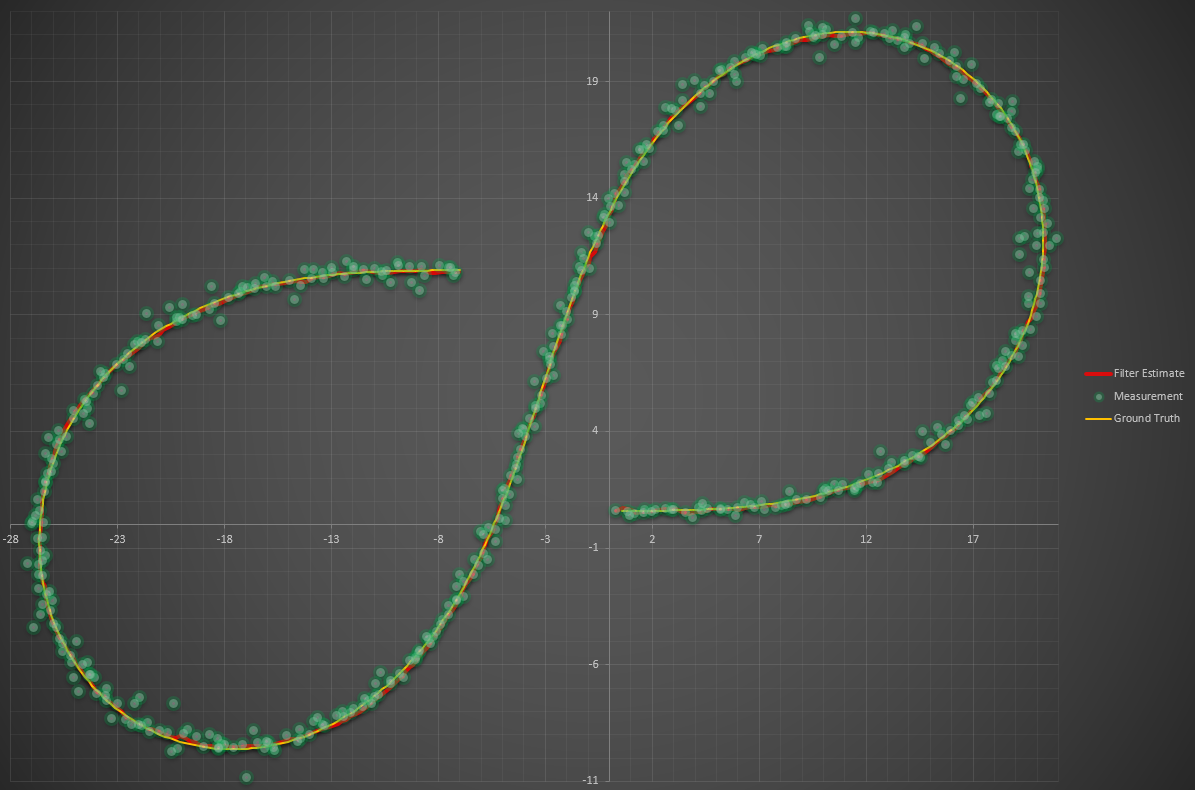
Zooming in on the lower left corner, here are a few different scenarios. First the full UKF:

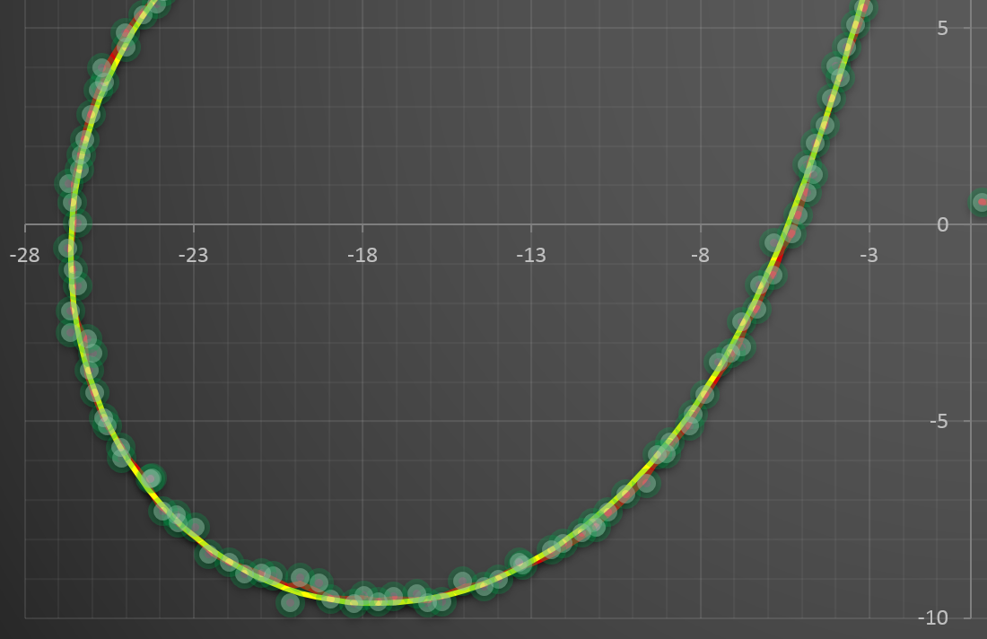
And next, using only LiDAR data:

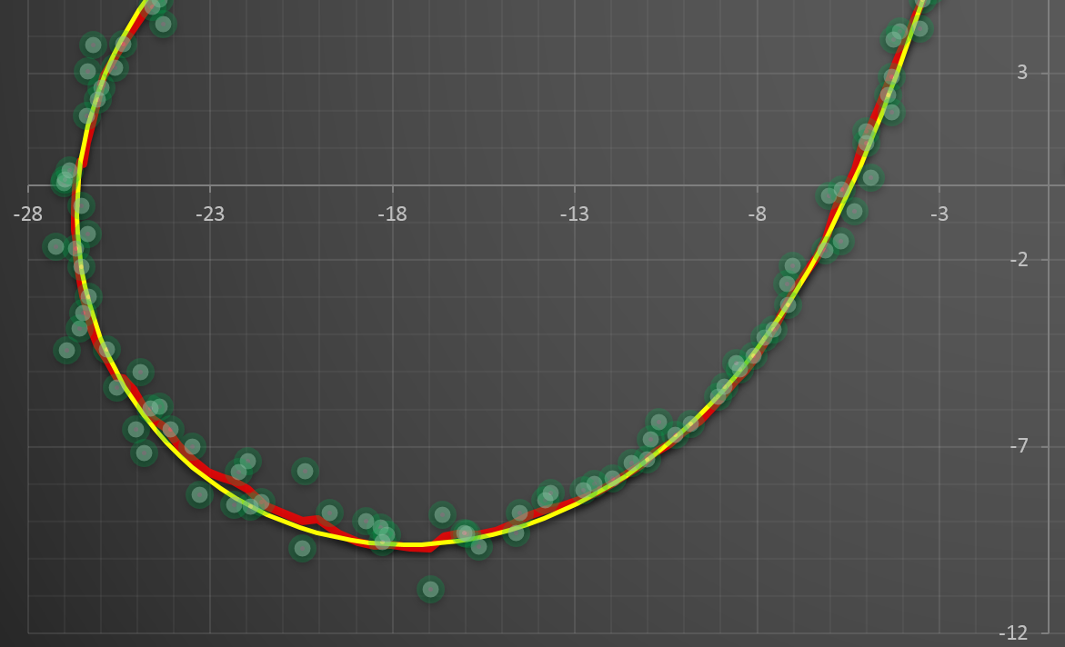
And finally, using only radar data:

The source code for this project is available on my Github here.