Udacity Self-Driving Car Nanodegree Project 5 - Vehicle Detection

Welcome to the “mom report” (Hi mom!); if jargon and mumbo jumbo are more your style then maybe this is what you’re after, otherwise enjoy!

…And just like that I’ve completed Project 5, and with it Term 1, of the Udacity Self-Driving Car Engineer Nanodegree - hooray! I’m already counting the days (eight, at the moment) until Term 2 begins and trying to decide the best way to sustain my momentum, starting with this here recap of Project 5 - Vehicle Detection.

The interesting thing to me about this project, in particular, was that it sort of occupied the middle ground between the first and fourth projects and the second and third projects. The first and fourth projects used old-school computer vision techniques and explicitly defined steps to produce an output (highlighting the location of lane lines), whereas the second and third projects employed deep learning’s hot-ass newness (I might have to trademark that) to sort of let the program figure out the rules on its own based on a ton of examples.

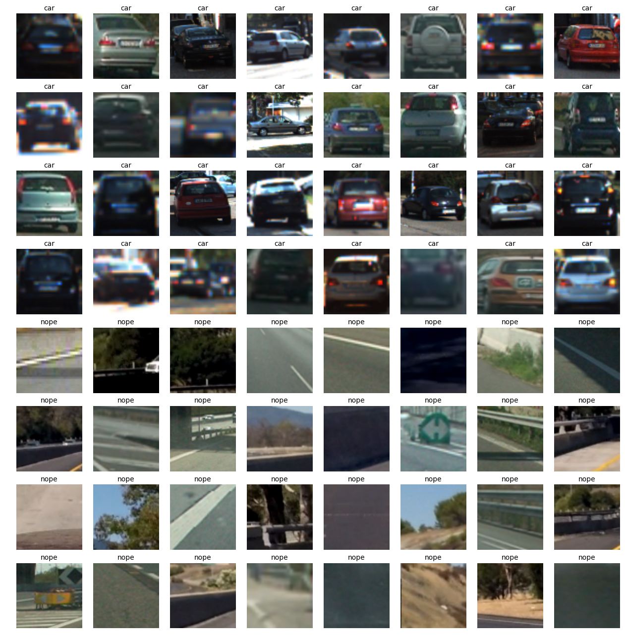
The goal of the Vehicle Detection project was to identify vehicles in dashcam video. While there are already deep learning implementations (e.g. YOLO and SSD) that utilize convolutional neural networks and can efficiently and reliably identify vehicles given a full video frame, our assignment was to use a more… classic approach - train a traditional machine learning classifier on images of cars and non-cars and then run a sliding window search on each video frame to identify the location of any cars. Here are some sample images from the dataset we were given to train our classifier with:

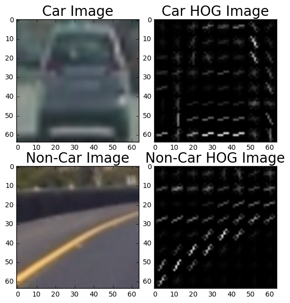
Now, training a classifier on raw image data is unnecessary and would probably take forever. There are better ways to extract features (wait, you mean we have to do that ourselves?!) from an image to train a classifier, and the lectures presented three: grouping color features into bins spatially (resize the image to something very small and flatten into a single list of values), histograms of color, and the Histogram of Oriented Gradients (HOG). Here’s an example of HOG features, which captures and groups the edges in the image (and happens to be popular for facial recognition):

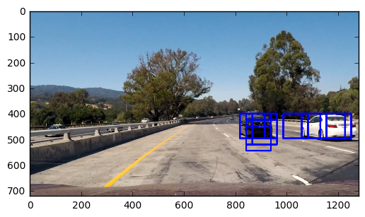
Using HOG features alone and a Linear SVM classifier, I was able to get 98.17% test accuracy on the dataset. I could have improved that by combining other feature extraction methods, but I figured an accuracy over 98% would be acceptable and in the interest of performance I carried on to the next step - the sliding window search. This involves running every square patch of the image (with some overlap) through the classifier to determine if there’s a car there or not. If the patch is 64 x 64 pixels and the overlap is 50%, that means around 850 patches of a 1280 x 720 image will be classified. Here’s what my first attempt at that looked like, using a 96 x 96 patch and 50% overlap:

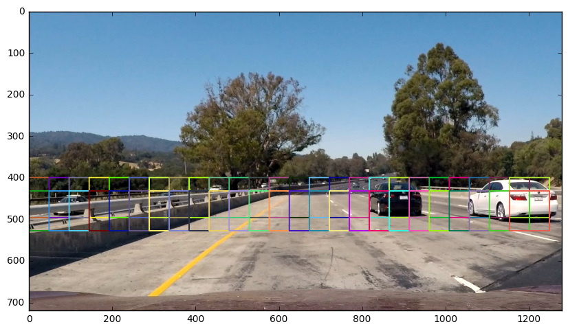
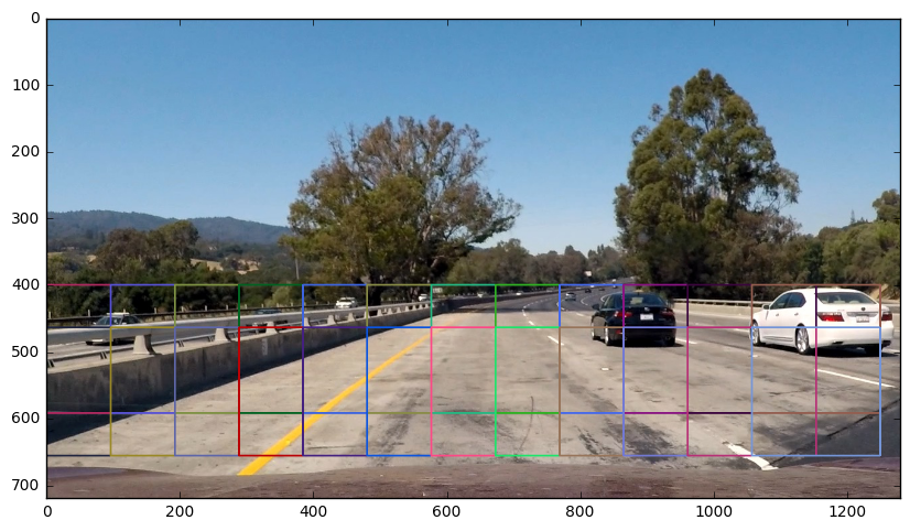
Actually pretty good! Still, there were improvements to be made. Foremost, obviously there aren’t going to be any cars in the sky (yet!) so that area of the image can be eliminated from the search, and cars near the horizon will be smaller than cars in the foreground. Here are the areas and window scales that I searched in the end, based on where I expect to find cars and at which size:

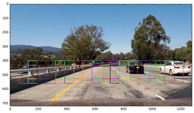
Searching each of those windows resulted in the following positive detections from the classifier:

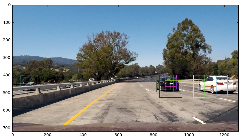
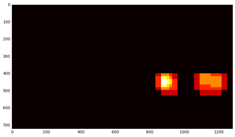
I think it worked! It even found a car in the oncoming lane. This test image might have just gotten lucky (particularly with that oncoming lane detection) - others tended to have more false positives, so the next step was filter these out. I began by creating a heat map and adding “heat” to areas where the classifier made a positive prediction - overlapping detections were given more heat. Here’s an example:

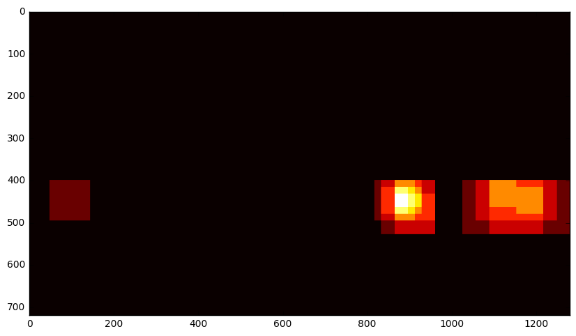
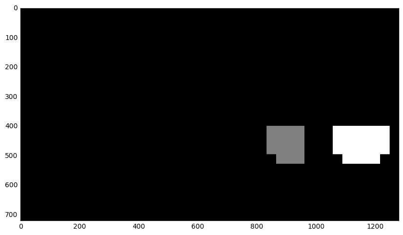
Since false positives tend to have only one or two overlapping detections, while true positives tend to have several, I applied a threshold to the heatmap and essentially turned off all of the weak spots:

Next, the handy label method from scipy.ndimage.measurements library conveniently groups the contiguous “on” pixels in the heatmap and gives each a label. The result looks like this:

From there, the bounding boxes for individual cars are determined by the bounds of the heatmap labels.

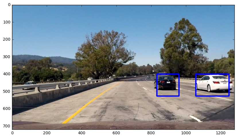
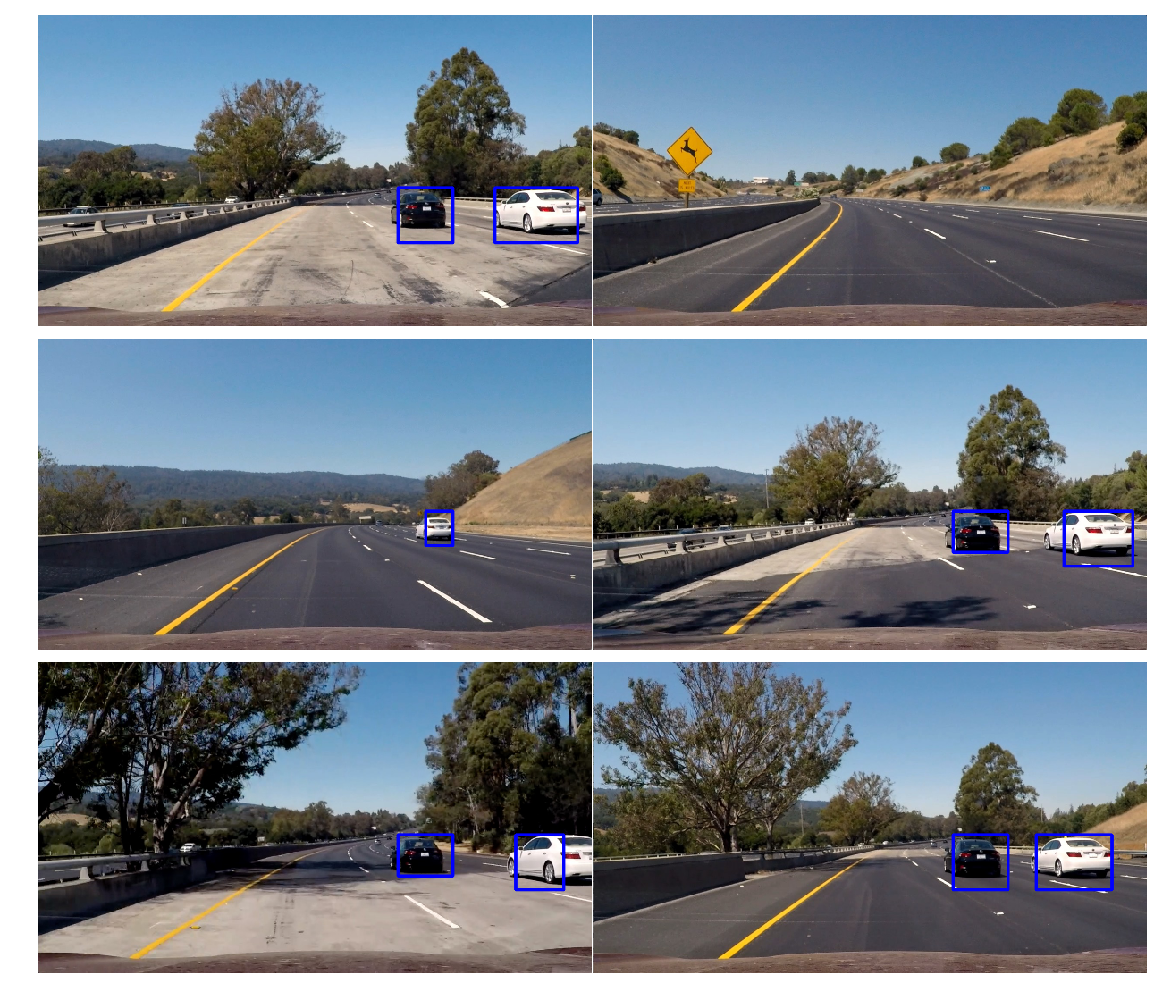
Done. And here’s the same pipeline on various other images:

The pipeline works well on individual images, but the real test was video. Taken as-is, the pipeline works well, but the bounding boxes are jittery, they sometimes disappear, and there are also occasional false positives. To alleviate this I averaged the heatmaps from the previous fifteen frames for each new frame of video, and set the threshold to an appropriate level. This produced the buttery smooth results below.

It’s still not perfect (for instance, it loses the white car for a few frames) but I’m happy with how it turned out. It doesn’t capture any oncoming cars, either, which is caused by the averaging over time certainly. I feel that a more sophisticated frame-to-frame tracking method would help (along with a higher-accuracy classifier and more overlap in the search windows) but it would also slow the pipeline down. Having seen what YOLO can accomplish, I’m thinking a deep learning approach is definitely the way to go.

Again, if it’s the technical stuff you’re into, go here.