Udacity Self-Driving Car Nanodegree Project 2 - Traffic Sign Classifier
Project number two in the can! (I realize now that that sentence might sound like toilet humor, but I swear it was unintentional.)
I’m truckin’ right along in my Udacity Self-Driving Car Engineer nanodegree program, as my personal mentor is well aware from our weekly check-ins. I feel bad for the guy because I honestly haven’t had much need for him. I’m glad he’s there, of course! But I guess the course content keeps everything pretty crystal clear, and the help from the community at large is a big heads-up to whatever obstacles might be coming my way (one benefit of being placed into a cohort that started later than others - December represent!). It’s good to know that Udacity has gone to great lengths to make sure I don’t get stuck.
That’s not to say that this thing is a cake walk by any means! I consider myself lucky that I really, truly enjoy it - that I’m eager to spend all of my scant me-time with my laptop open training a neural network. Otherwise, I think it would be easy to fall behind. Udacity estimated that students would need to devote ten hours a week to the curriculum. It’s hard to gauge since I’m currently a week or two ahead of schedule, and I’m sure it depends on your skill level coming in, but I’d be inclined to bump those ten hours up at least fifty percent. We’ll just have to see how the rest of the term goes, but for now…
Project 2: Traffic Sign Classifier
This unit was all about deep learning, and there was a boatload of lecture and exercise material leading up to the project. I found myself glad that I’d taken Udacity’s Intro to Machine Learning and Deep Learning classes ahead of starting the nanodegree. A hefty chunk of the Deep Learning course material made an encore appearance in the nanodegree curriculum, but I can’t complain - the course was short and dense, so it was good to take a second look at it.
So what is deep learning, anyway? That’s the million dollar question, my friend.
The truth is, the jury is still kind of out on deep learning. Why? Well, mostly because the academic community hasn’t quite nailed down how it works. It just kind of does. At its core is a concept (an algorithm, I suppose) called a “neural network” which is a combination of basic units called “perceptrons,” each of which simply takes a number of inputs, multiplies each input by a chosen weight and adds a chosen bias, and produces an output. A perceptron with a one-dimensional input will produce a line (think mx+b from algebra class), which can be used to fit data points with continuous outputs (i.e. a “line of best fit”) or divide data points with discrete outputs (i.e. classes, like “short” versus “tall” if your input were height in inches, for example). Combine enough of these perceptrons in some configuration and you can come up with insanely complex models for predicting the output of a given input. Clear as mud?
But wait, how do you figure out what those weights and biases should be? Well, you let the computer do that for you. (Handy little things, ain’t they?) For that you need data. A lot of data. And not just that, each piece of data needs to be labeled. But then, if you configure your neural net sufficiently, the computer will magically (Really! … OK, not really.) produce weights and biases that can correctly guess the output for an input it’s never seen before. Super cool!
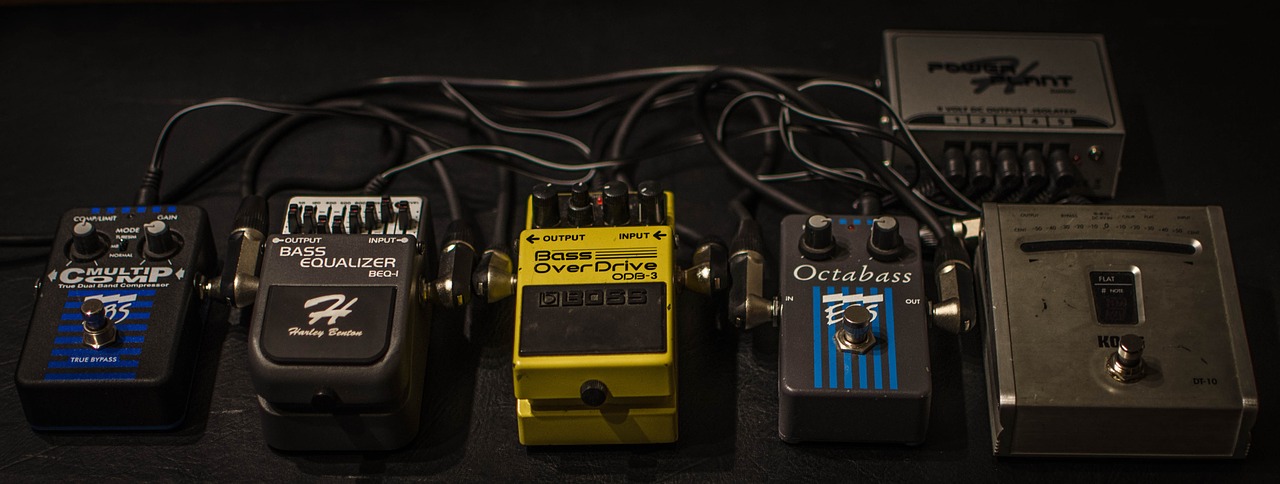
I tried to think of an analogy to describe this, and here’s the best I could come up with: Think of a guitar player’s setup - with the guitar and amp and a bunch of pedals to shape the sound of the guitar. Now imagine you’re trying to replicate Annie Clark’s sound, and you’ve got the guitar and the amp and all the pedals set up the same way she does, but you can’t tell from your crappy low-res photos what numbers all those knobs are dialed to. What now? Deep learning would be like taking a recording, giving your computer the inputs (chords and notes being played) and the outputs (sounds coming out of the amp), and letting it figure out how to dial in all of those knobs. (Be warned, this analogy is very fragile and its feelings are easily hurt.)
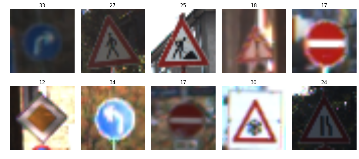
For this project, the image data came from the German Traffic Sign Detection Benchmark (GTSRB) data set. Here are some sample images (you can see the numerical labels above each image):
The project was implemented as a Jupyter notebook (with plenty of helper code already filled in). The higher-level steps prescribed to complete the project were:
- Load the Data
- Dataset Summary & Exploration
- Design and Test a Model Architecture
- Test a Model on New Images
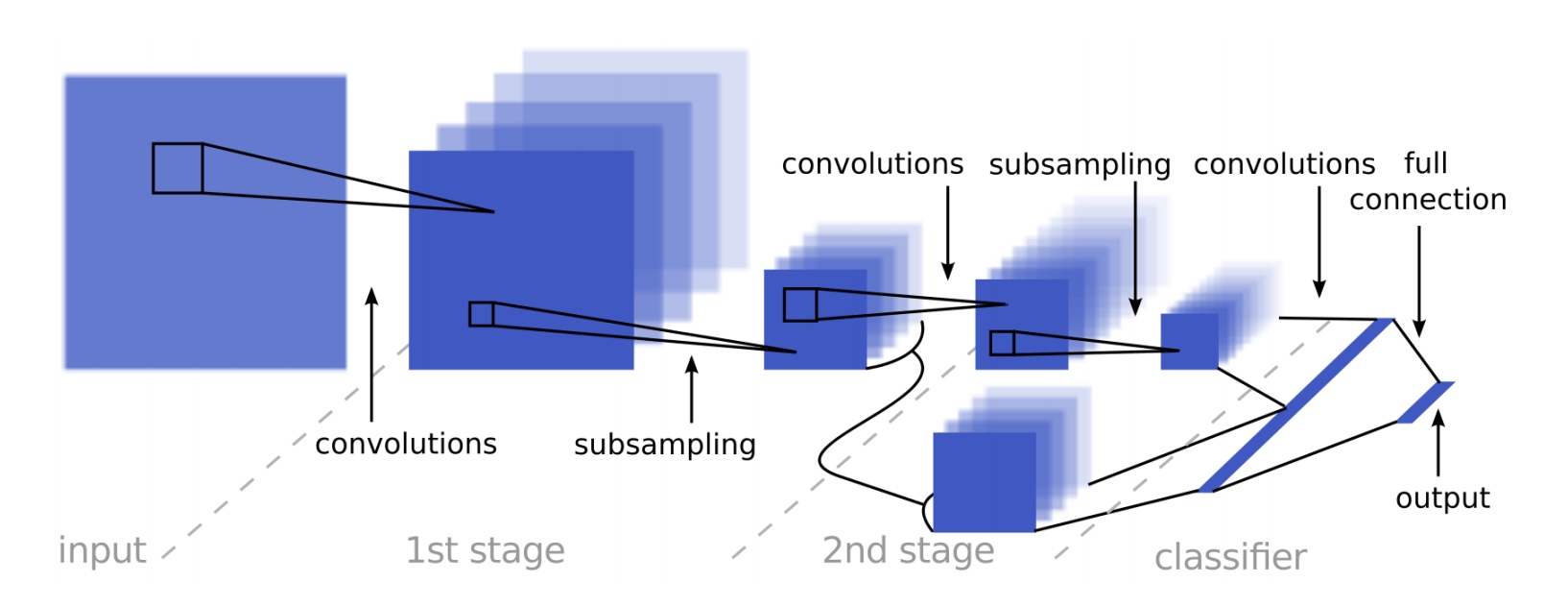
A previous exercise introduced the LeNet architecture, cleverly named for Yann LeCun who developed it in 1998 to classify images of handwritten digits zero through nine. Even though we are classifying traffic signs, not handwritten digits, the assignment suggested using LeNet as a starting point. Indeed, it performed quite well - achieving 96.5% validation accuracy right out of the box.

Udacity also recommended reading a journal article written by Pierre Sermanet and (wouldn’t you know it) Yann LeCun, describing a neural network-based approach specifically for… wait for it… classifying traffic signs! Score! I was eager to implement this new architecture and see how it performs. Even though some of the specifics of the architecture were left out of the paper, I took a stab at it and filled in the blanks so as to keep it as similar to LeNet as possible.
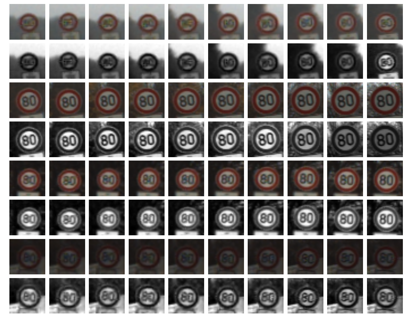
Switching to this architecture immediately netted me another 1% validation accuracy (now 97.5%), but why leave it at that? The paper also describes other strategies for improving accuracy, including converting the image to grayscale, “normalizing,” and augmenting the data by copying and slightly modifying underrepresented classes. I implemented all of these, plus a technique called “dropout,” to improve validation accuracy another percent or so.
Augmentation was by far the most time-intensive strategy to carry out, but it was also said to be one of the most important to achieve stellar accuracy. Prior to augmentation, the number of data points (images) per class looked like this:
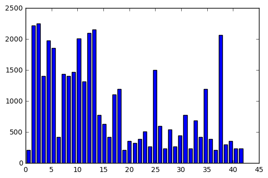
Some of the classes were represented far more than others, in some cases by more than a factor of ten! This is a problem for a machine learning algorithm, because the lack of balance in the data will lead it to become biased toward the classes with more data points. If I give you a hundred stop signs, a yield sign, then two hundred more stop signs, what do you think is going to come next? One solution would be to throw out data from the more heavily represented classes, but hang on there just a second pardner! That’s perfectly good data you’re tossing out. Better idea: generate more data points for the less represented classes.
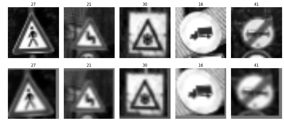
My approach to augment the data was to loop through each class, 1 through 43, and if there were less than 800 samples from that class I then looped through each image of that class generating “jittered” copies until there were 800 samples total. The jittering process consisted of applying a small but random vertical and horizontal shift, a small but random scaling factor, a small but random amount of warping, and a small but random adjustment to the brightness of the image. Everything is “small but random” because I wanted to be careful not to produce an unrecognizable image. If it doesn’t look like a stop sign any more and I still classify it as a stop sign it’s just going to confuse my model. Here are a few examples of the results from this process:
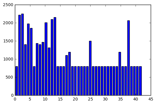
This process took around thirty minutes to run on my home computer, but afterwards the number of data points per class looked like this:
From this point the only thing left to do was to fiddle with the training “hyperparameters” to produce a model that achieves the best possible validation accuracy. This is where running on a GPU (thanks to a Udacity-supplied credit to Amazon Web Services) came in handy. The model training process can be tedious, and generally took about five minutes on my home computer. AWS cut this down to about one minute, allowing me to try several combinations of hyperparameters. In the end, my model attained over 99% validation accuracy.
Now that I was satisfied with my model it was time to evaluate it against a “testing” portion of the data set. This data had been put aside from the beginning because the model can become biased toward the data used to determine validation accuracy, sort of through my eyes, strangely. The test set helps to determine how the model performs against “new” data that neither I nor the model has seen. My testing accuracy came out right around 95% - pretty good!
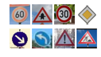
And now for a little extra fun - we were instructed to find at least five images of traffic signs, around the internet or in person, and see how our model performs on those. Here are the eight that I chose:
And here’s how the model performed on them:
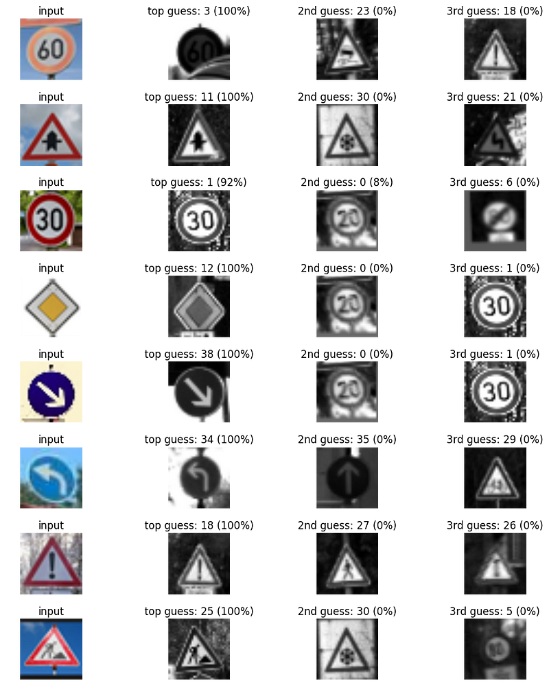
Rather than just show the predicted class number for each sign, I pulled an example from the original dataset. Shown are the top three predictions and (in parentheses) the certainty of each prediction.
Wait… a hundred percent? Seriously? I don’t know how this model can be that sure of its prediction. Granted, I gave it some real softballs, there. But still, I would have expected them all to be in the 75-90% range. Whatever - I’ll take it! Good job, model!
At this point there are still a few things I could experiment with. For example, I never ran color images through the model because I was trying to save myself time and processing power in the beginning, but the grayscale performed really well (as Sermanet-LeCun indicated) so I never bothered. I never played around much with the jittering parameters, either. I could probably think of a dozen different ways to further experiment, but you have to stop somewhere… and I have a “behavioral cloning” project coming up that’s got me frothing at the mouth.
My completed Jupyter notebook for this project can be found on my GitHub