Udacity Self-Driving Car Nanodegree Project 11 - Path Planning - Part 1

The first project in Term 3 of the Udacity Self-Driving Car Engineer Nanodegree program, and the eleventh (!) overall, is Path Planning. I can’t believe it’s been almost two months since I wrote the Model Predictive Control blog post. I guess the few weeks between terms, few weeks while the Path Planning project was being finalized, and few weeks it took me complete this project do add up to a couple of months.

Let me start by saying, this project was a beast… a beast of my own creation, I suppose. I consider it a success and a failure. As I mentioned previously and will go into more detail below, I kept at a more complex solution longer than I should have. The theme of my progress throughout this Nanodegree and, to a certain degree, life over the past year has been: triage. I’ve been continually juggling Nanodegree project deadlines, regular blog posts, job search activities, and all the other stuff (work, laundry, dishes, toddler bedtime, etc.) to mostly good results, managing to stay organized and prioritized. Nanodegree deadlines always had top priority, but finishing a blog post might take priority over an optional stretch goal, for example. This time, though, stubbornness got the best of me - I followed this rabbit just a little too far down the hole.

Let’s take a step back, though. The other functions of self-driving cars that we’ve covered so far - object detection and tracking, sensor fusion, localization, and control - operate at a lower level. Path planning is what ties them all together, connecting the data interpreted from the sensors and producing a trajectory for which the control system can decide how to apply gas, brake, and steering. The path planning function can be broken down into three parts - prediction (as in, predicting the behavior of obstacles including other cars), behavior planning (deciding which action to take, at a high level, in order to reach the goal safely, efficiently, etc. - e.g. slow down, speed up, turn, self-destruct), and trajectory generation (translating that behavior decision into a path - a set of points or a formula - for the control system to implement).

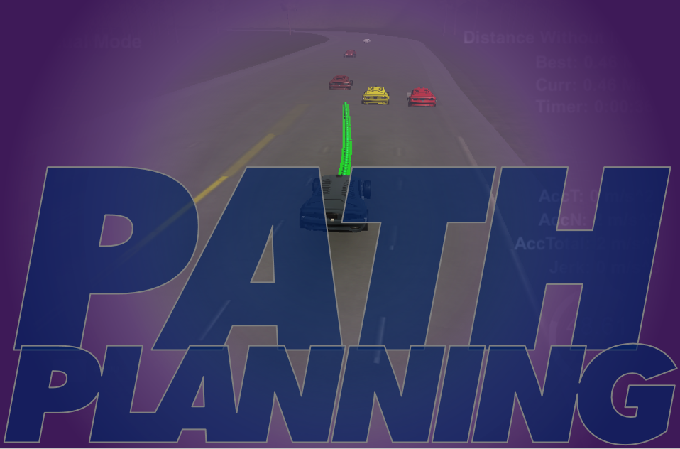
This project again put the Udacity simulator to use, this time in a highway driving scenario. The goal is to drive the entire 4.32 mile length of the gently curvy, closed-loop track at near the posted speed limit while navigating traffic and without any “incidents” to include: driving over the speed limit, exceeding limits on acceleration and jerk (i.e. the change in acceleration over time, which can make for an uncomfortable ride), driving outside of the lanes, and, of course, colliding with other cars. The simulator expects of us a list of (x,y) map coordinates, each of which our car will obediently visit at twenty millisecond intervals (even if that means violating every law of physics). In return, the simulator provides us with telemetry data for our car (position, heading, velocity, etc.), sensor fusion data for the other cars (at least the ones on our side of the highway), and whatever points of our previous path the car hasn’t already visited. We are also provided a .csv file with a list of track waypoints. We can then use this data to determine a trajectory, convert it to a set of x and y points, and tack these points onto the end of however many points of the previous path we’ve decided to keep (this can help to account for latency between our planner and the simulator and, if you’re like me, it can also serve to artificially smooth the transition to a new trajectory).

The project instructions included a couple of simple example trajectories: driving in a straight line at a constant speed, and driving in a circle at a constant speed - with no consideration for comfort or other cars whatsoever. From there we were on our own. I took a page from previous projects and scoured the lesson material for code snippets that I could incorporate into my planner. Unlike so many previous projects, there was very little that I could just copy and paste as-is. Much of the lesson material required some sort of translation, be it from Python to C++, from a one-dimensional to two-dimensional domain, or from a discrete to continuous domain.

My implementation, at least the first go-around, looked something like this:

1. Interpolate the waypoints for a nearby portion of track (this helped to get more accurate conversions)
2. Determine the state of our own car (the position, velocity, and acceleration projected out a certain amount of time based on how much of the previous path was retained)
3. Produce a set of rough predicted trajectories for each of the other vehicles on the road (assuming a constant velocity)
4. Determine the “states” available for our car (in this case, “keep lane,” “change lanes to the right,” or “change lanes to the left”)
5. Generate a target end state (position, velocity, and acceleration) and a number of randomized potential trajectories (with elements of the target state perturbed slightly) for each available state (these “Jerk-Minimized Trajectories” (JMTs) are quintic polynomials solved based on our current initial and desired final values for position, velocity, and acceleration)
6. Evaluate each of these possible trajectories against a set of cost functions (rewarding efficiency and punishing things like collisions, higher average jerk, or exceeding the speed limit, for example)
7. Choose the best (i.e. lowest-cost) trajectory
8. Evaluate it at the next several 20-millisecond intervals
9. Tack those onto the retained previous path, and
10. Return the new path to the simulator

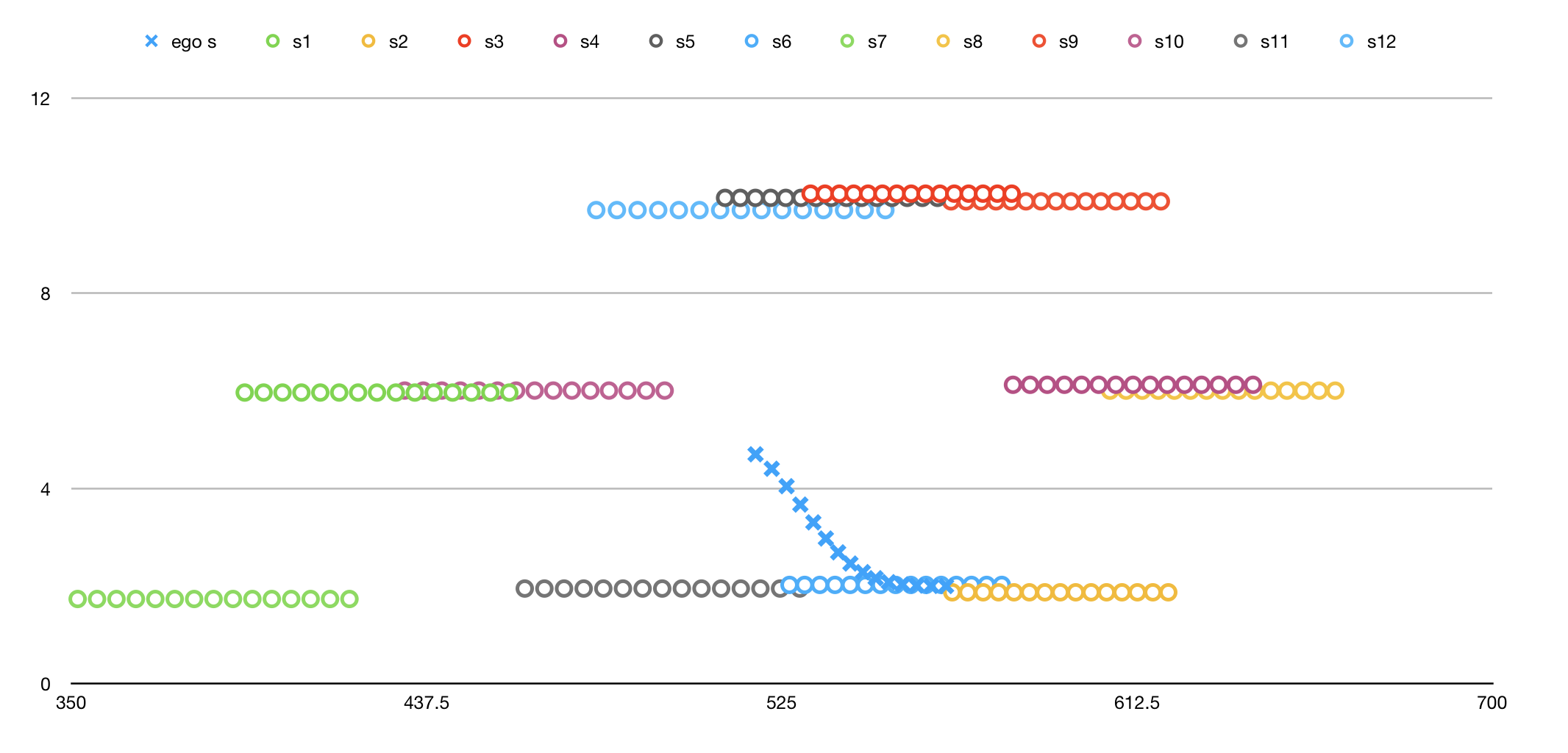
The image below is a visualization of predicted trajectories for other vehicles on the road, as well as the “ego” vehicle (in blue x’s) mid lane change.

It took some time to achieve a successful build of the code, and more still to simply get the car to move. From there it was several days of fighting to get the car to drive even halfway decently. I had hit a roadblock. I bit off more than I could chew, and even after throwing out the fancier bits and just sticking to a single target and trajectory, keeping to the middle lane, and ignoring other traffic, my car was still jerking and wavering at best and flying madly to all corners of the track at worst. I believe the issue was primarily in stitching together the previous path with the newly generated trajectory and giving the planner an accurate state (both beginning and end) from which to build the trajectory. It didn’t seem to have trouble with the initial trajectory and, indeed, the car seemed to start off fairly well in that first fraction of a second, but from there it would invariably violate the acceleration and jerk limits before either settling into a somewhat constant velocity or just taking off like a damn rocket.

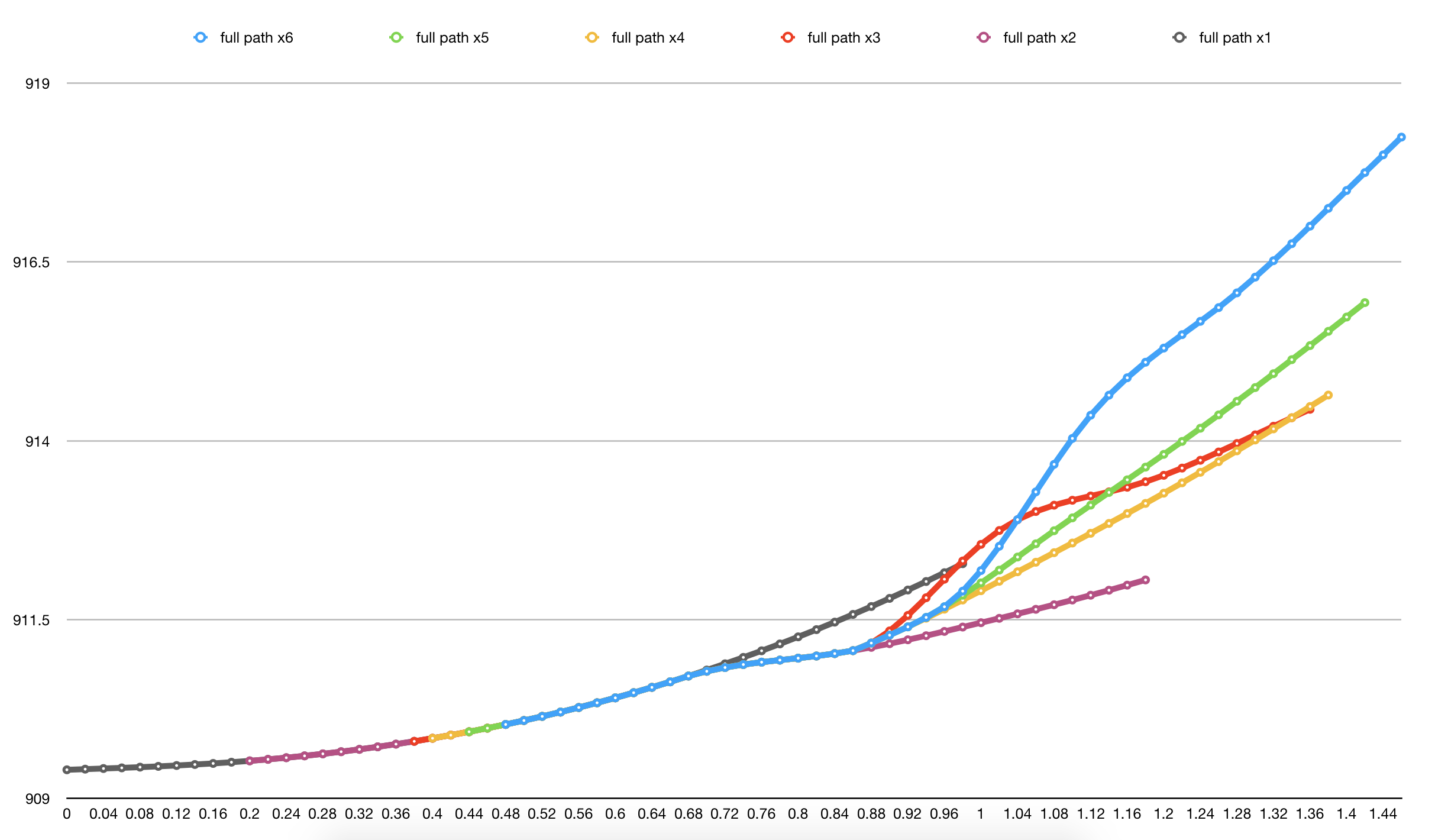
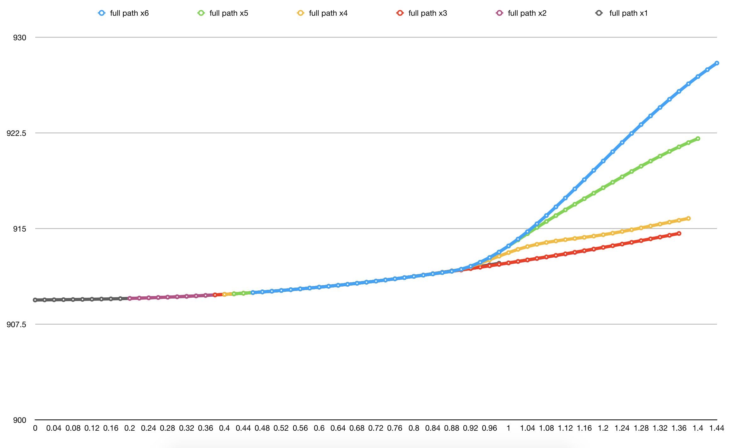
These images below show some of the paths my planner was passing to the simulator, for each of two different methods (which I won’t go into here) I tried for determining the starting parameters of the JMT. You can see that in both cases the first trajectory is smooth, but subsequent trajectories diverge at the point where points from the previous path are no longer retained:

I was going mad. I couldn’t sleep. I would come up with a fix, but one problem always seemed to lead to another. And even now I’m convinced that there was just some little thing that I was missing - some simple tweak that would do the trick. Meanwhile Udacity released a walkthrough that put very little of the lesson material to use. It was simple. Too simple. Yet, after two weeks of battling with a more robust approach, I decided to abandon much of my approach and adapt it to the simplified approach in the walkthrough.

…and that’s where I’ll pick it up next week in part 2

The code for this project, as well as a short but more technical write-up, can be found on my GitHub.