Udacity Self-Driving Car Nanodegree Project 10 - Model Predictive Control

The tenth project for the Udacity Self-Driving Car Engineer Nanodegree Program, and the final for Term 2, was titled “Model Predictive Control” (MPC). MPC takes the concepts of PID control to the umpteenth level, and with it comes umpteen times the complexity. Though, Udacity unloaded much of that complexity to the IPOPT and CPPAD packages.

Like the PID control and Behavioral Cloning projects, the goal of this project is to navigate a track in a Udacity-provided simulator. I’m glad to see them getting some extra mileage out of the “lake” track (get it?). All three projects require our code to communicate with the simulator via websocket, sending it steering and throttle commands, based on data it provides. In behavioral cloning it provides a camera feed, in PID control it’s cross-track error (CTE, roughly the distance from the track center line), and this time it provides telemetry (position, velocity, heading) and a few waypoints for the coming stretch of track. This project’s bonus challenge turned out to be a mandatory (what?!): once we’ve got our controller working we have to throw in a 100ms delay before sending our control commands, to simulate the type of latency we might encounter in the real-world.

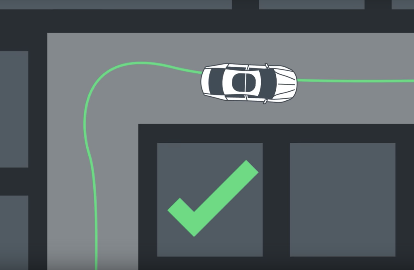
The first order of business is to fit a curve to the provided waypoints, preferably after they’ve been transformed from the track coordinates to the vehicle’s viewpoint to simplify future calculations. I’ll call this the curve of best fit. Then the IPOPT and CPPAD packages can be used to calculate an optimal trajectory and its associated actuation commands in order to minimize error with the best fit. You might think, “Well, why not just follow the best fit?” Well, sure - that’s sort of what we did in PID control, but now we have the benefit of knowing what’s coming and can plan our controls a little more cleverly. When you make a turn in your car, you don’t exactly take it at ninety degrees, do you? Maybe something more like this?

MPC can take a vehicle’s motion model into account to plan out a path that makes sense given a set of constraints, based on the limits of the vehicle’s motion, and a combination of costs that define how we want the vehicle to move (such as staying close to the best fit and the desired heading, or keeping it from jerking the steering wheel too quickly).

The optimization considers only a short duration’s worth of waypoints, because that’s all we really need to plan for (as far as our actuator controls are concerned). We can tune the number of discrete points in time that the optimizer uses in its plan, as well as the time gap between them, so it can compute the best plan within a reasonable amount of time (we certainly want it fast enough to control the car in real time). The optimizer requires a massive one-dimensional vector that includes state variables and constraints on each for each time step in the plan, along with the overall cost function - not particularly intuitive, to be frank, but manageable.

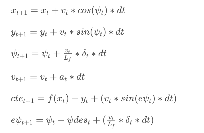
Since the variables for future time steps depend on previous time steps, their constraints make use of vehicle’s kinematic model. The kinematic model includes the vehicle’s x and y coordinates, orientation angle (psi), and velocity, as well as the cross-track error and psi error (epsi). Actuator outputs are just acceleration and delta (steering angle). The model combines the state and actuations from the previous time step to calculate the state for the current time step based on the equations below:

After some debugging and tuning the cost function, my car was making its way around the track. It was time to tear it all down by adding the latency - and that’s just what happened. My approach to dealing with it was twofold (not counting simply limiting the speed): the original kinematic equations depend upon the actuations from the previous time step, but with a delay of 100ms (which happened to be my time step interval) the actuations are applied another time step later, so I altered the equations to account for this. (Note: my project reviewer suggested a simpler solution - projecting the car’s current state 100ms into the future before even running the MPC Solver method. As it stands, for example, my car’s x and y position as passed to the solver is [0,0] (its current position, from its own viewpoint), but 100ms later it should be different.) Also, in addition to the cost functions suggested in the lessons I incorporated a cost penalizing the combination of velocity and steering, which resulted in much more controlled cornering.

Here’s a little lighthearted video review of the whole experience:

The source code for this project can be found on my GitHub